Climatologists and economists all agree – climate change is a threat to future economic performance and one of the major structural problems the global economy is facing (Blanchard and Tirole 2022). The literature has indeed shown that, in recent decades, rising and volatile temperatures significantly reduced GDP, with advanced countries like the US being no exception. This poses challenges for governments to design appropriate policies in response to uncertain climate outcomes and coordinate their efforts across countries.
The urgency to arrest climate change has also fueled a debate among central bankers about what they can do to support the fight (e.g. Boneva et al. 2022, Hartmann et al. 2022, Masciandaro and Russo 2022). However, while the discussion rests on the potential repercussions of climate-related phenomena on the central bank’s activity and, in particular, on the conduct of monetary policy, it generally lacks solid empirical grounding. This depends on the fact that the joint effects of climate on economic output and consumer prices, as well as the correct monetary policy response, are open issues. Since unfavourable temperatures can have both supply-side effects (for example, by decreasing labour productivity) and demand-side ones (for example, by changing consumption patterns or diverting capital to increase climate resilience). Therefore, it is not clear, a priori, what the overall price response to temperature variations could be and, consequently, whether and how monetary policy should react to them.
My recent paper (Natoli 2022) takes up this issue by quantifying the impact of temperature oscillations on the US economy. I study how GDP, private consumption, and investment are affected, how the CPI index responds, and, in turn, how these effects propagate to short- and long-term interest rates on government bonds. For this purpose, I propose a new way to identify unpredictable changes in temperatures that fit with the notion of a shock in macroeconomics.
Constructing temperature shocks
Temperature shocks have been constructed using daily average temperature data for each US county since the 1970s. Quarterly county-level temperature ‘surprises’ are computed as the difference between the number of highest and lowest temperature days within the quarter and those observed in the same county during the same quarter of the past five years. The rationale is that, based on their most recent experience, agents learn over time about the set of prevailing temperatures in each season, updating their beliefs every year. If the number of seasonal highs and lows in one quarter exceeds expectations, it represents a positive – expected to be economically harmful – surprise. By focusing on the size and persistence of temperature variations and by identifying exogenous changes with respect to the most recent temperature levels, this approach stresses the idea that unexpected exceptionally hot and cold weather is what matters in the short run. It therefore overcomes some of the flaws of standard methods used in the literature based on positive versus negative temperature variations – which can potentially mix good and bad economic shocks – and identification based on actual variations with respect to historical temperature averages – which misses the continuous adaptation of agents to the increasingly frequent temperature extremes.
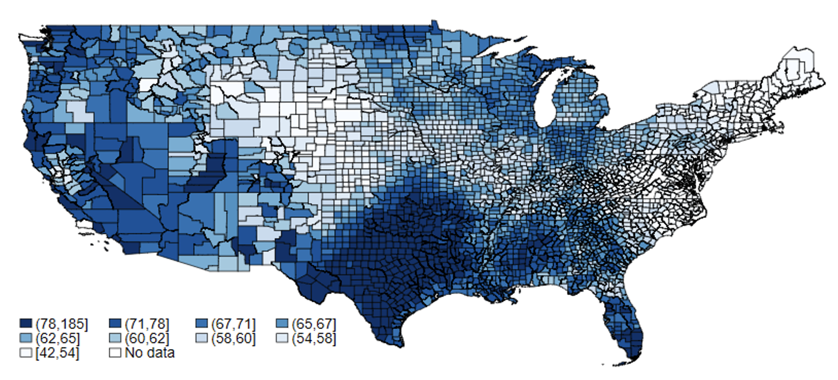
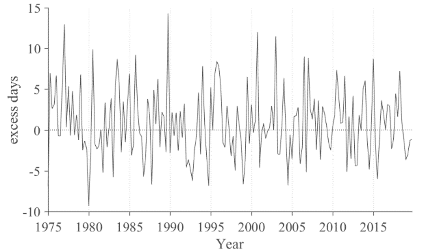
County-level surprises are then aggregated to obtain a US-wide temperature shock. Figure 1 displays the incidence of surprises by county (panel a) and the evolution over time of the US-wide temperature shocks (panel b). The first picture reveals that, between 1975 and 2019, surprises were largest in southern and western counties; the second picture shows that, at the national level, adjustments in the shape of the temperature distribution were largest – inducing bigger shocks – in the early part of the sample than in recent times. This does not imply that temperature fluctuations have declined in size, but simply that extreme temperatures have become more the normality in recent times, so less surprising than in the past.
Figure 1 County-level temperature surprises and US-wide temperature shocks
(a) The average size of county-level surprises
(b) US-wide temperature shock
The effects of temperatures on the US economy and monetary policy
The constructed US-wide shock is then used to study the average response of key economic variables to temperature variations between 1975q1 to 2019q4, using local projections (Jordà 2005). Figure 2 shows the impacts on the US economy up to 16 quarters after the shock: exceptional temperatures have a negative effect on GDP, which increases over time reaching a trough after 2 years, in line with Lemoine (2021), with a strong impact coming from private investment. Moreover, shocks reduce the Consumer Price Index (although with a lag), suggesting that demand-side effects are predominant. Temperatures also induce a significant reaction by the Federal Reserve, displayed in Figure 3: in line with the response of GDP, the Fed’s economic nowcast (produced within the set of Greenbook Forecasts) are also revised down, tracking the downturn as time passes (the first picture). This induces an expansionary monetary policy reaction as short rates also fall, with effects spreading out to the long end of the yield curve (the second and third picture). While the behaviour of interest rates is not by itself a guarantee that the Federal Reserve correctly identified the source of the downturn, some evidence points to an increase in the Fed’s attention to temperature fluctuations. Indeed, the occurrence of temperature-related wording in the transcripts of individual FOMC meetings slightly increases after adverse temperature shocks (the fourth picture).
Figure 2 The effects of temperatures on the US economy, up to 16 quarters after the shock
Figure 3 Federal Reserve reaction, up to 16 quarters after the shock
All in all, these findings suggest that climate-related shocks have concurred to influence the conduct of US monetary policy during the last 50 years, adding a piece of evidence to the debate on the role central banks can play to counteract the economic effects of climate change. The technique used to construct the US temperature shock can be applied to other economies and serve as a reference to obtain other weather-related shocks under the same logic.
References
Blanchard O, J Tirole (2022), “Major future economic challenges”, VoxEU.org, 21 March.
Boneva, L, G Ferrucci and F P Mongelli (2022), “To be or not to be ‘green’, part 1: Why climate change is relevant for monetary policy”, VoxEU.org, 17 June.
Hartmann, P, A Leonello, S Manganelli, M Papoutsi, I Schnabel and J-D Sigaux (2022), “Central banks, climate change, and economic efficiency”, VoxEU.org, 10 June.
Lemoine, D (2021), “Estimating the economic impact of climate change from weather variation”, VoxEU.org, 9 July.
Masciandaro, D and R Russo (2022), “Central banks and climate policies: Unpleasant trade-offs are likely”, VoxEU.org, 18 July.
Natoli, F (2022), “The macroeconomic effects of temperature surprise shocks”, available at SSRN


